THE MAXIMORUM GDELT PROJECT

Our product leverages the GDELT event dataset and the Self-Organizing Maps (SOM) model to develop a comprehensive optimization system for supply chain procurement decisions. The SOM model detects adverse movements in specific countries, serving as an anomaly detector, and the results are used as a proxy to measure the risk of having problems with the supply chain in those countries. This risk assessment is integrated with cost considerations, enabling businesses to make informed sourcing decisions that balance cost efficiency with the potential risk of supply chain disruption due to social unrest or other adverse events. By combining advanced anomaly detection with real-time global data, our solution safeguards supply chains from unforeseen challenges in the international market.

Make production choices considering not only operational costs but also the lowest risk of social instability in the country

Technical Report

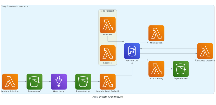
The ETL pipeline was created using AWS ETL tools. The process begins with a Lambda function that retrieves a list of all files from the GDELT website. It then compares this list with a manifest that contains all previously downloaded files. The function proceeds to download only the files that are not in the manifest and stores them in the bronze bucket.

Data Engineering

Data Extraction

Data Transformation

Data Governance

The second stage of our pipeline is the transformation process, where we use AWS Glue to unzip the files and send them to an unzip folder. AWS Glue was chosen because Lambda functions have limitations in terms of processing time and memory. Although AWS Glue is slightly more expensive, its cost is still not prohibitive for the pipeline.

To ensure data integrity, we chose to use AWS Redshift as our Data Warehouse. Once the Lambda function has finished downloading data from the GDELT website, it updates its own manifest and also updates a data injection manifest for the Data Warehouse, marking the newly downloaded files as pending for transfer to the DW. Another Lambda function, called "injection," is then responsible for checking which files are in this manifest, performing preliminary data validation, and subsequently sending the validated files to the Data Warehouse. After the injection process is complete, the function resets the injection manifest to prepare for the next batch of data.

After examining the database, we identified six variables for constructing the risk model: totalmentions, totalsources, totalarticles, medianavgtone, mediangoldsteinscale, and EventRootCode. We filtered the data by EventRootCode values of ('6', '7', '13', '14', '15', '16', '17', '18', '19', '20'). The definitions of these EventRootCode categories from the GDELT database are as follows:

- 6: *Coerce* - Events involving force or pressure to achieve compliance.

- 7: *Express Intent to Cooperate* - Statements or actions indicating a willingness to cooperate.

- 13: *Protest* - Demonstrations of disapproval or dissent, typically against something.

- 14: *Exhibit Force Posture* - Actions or displays intended to show force or strength, usually as a deterrent.

- 15: *Reduce Relations* - Actions aimed at diminishing or downgrading the relationship between entities.

- 16: *Demand* - Issuing a request or requirement with an expectation of compliance.

- 17: *Disapprove* - Expressing disagreement or opposition.

- 18: *Reject* - Refusal to accept, consider, or agree to something.

- 19: *Threaten* - Issuing warnings or expressing intentions to cause harm or take adverse actions.

- 20: *Engage in Unconventional Mass Violence* - Large-scale violent acts that deviate from standard or traditional methods of conflict.

We noticed that the series totalmentions, totalsources, totalarticles, medianavgtone, and mediangoldsteinscale had missing data points due to daily aggregation. To address this issue, we opted to work with weekly data, which allowed us to avoid dealing with missing values and ensured a more robust analysis for the risk model.

Data Analysis

Data Quality and Cleaning Process

Exploratory Data Analysis

During the analysis of these series, we observed that they become stationary after one or two differentiations. Although we have long time series, the volume is not sufficient to train more complex models such as Recurrent Neural Networks (RNN) or Long Short-Term Memory (LSTM) networks. Therefore, we experimented with traditional ARIMA models and found that the results were quite positive. Consequently, we decided to use ARIMA models to forecast these six variables for the following week.

Relevant Insights for Stakeholders

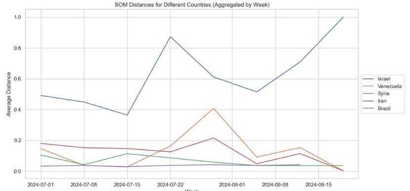
The figure below shows predictions for the next 8 weeks, generated using the following approach: we calculated a Self-Organizing Map (SOM) using all available historical data based on the six selected variables. We then used the last 10 months of this series to predict the value for the next week. This predicted value was subsequently used to calculate the distance between the predicted value and the SOM clusters. The greater the distance, the more the country deviates from typical behavior.

As illustrated in the image, countries like Iran, Israel, and Venezuela exhibited significantly distinct behavior compared to Brazil and Syria, indicating that these countries are farther from the norm and may warrant closer monitoring.

The development of this solution did not require extensive investment in feature engineering. By aggregating the totalmentions, totalsources, and totalarticles series, we achieved satisfactory results in handling the time series data. The only transformations we applied were calculating the median for the goldsteinscale and avgtone variables. These simple yet effective steps allowed us to maintain the integrity of the data while optimizing the performance of the time series models.

Machine Learning

Featuring Engineering

ML Modeling Tuning and Selection

The choice of Self-Organizing Maps (SOM) was driven by its effectiveness as an unsupervised technique for anomaly detection. We calibrated the model using various time series lengths, ranging from 10 months to 8 years, to find the optimal configuration. Before settling on SOM, we experimented with several clustering approaches, but none delivered the same level of performance. The SOM method provided a more reliable identification of patterns and anomalies in the data, making it the preferred choice for our analysis.

Model Deployment

Since the SOM is a lightweight and relatively easy-to-train model, we utilized an AWS Lambda function for the training process. After training, we serialized the model using Pickle and stored the serialized model file in an S3 bucket, enabling easy access and use by other functions responsible for calculating risk.

We also considered using AWS SageMaker for model deployment, but given the simplicity of the model, we determined that this approach would be over-engineering. The Lambda-based solution provided a more straightforward and efficient deployment process, aligning well with the project's requirements.

Model Optimization

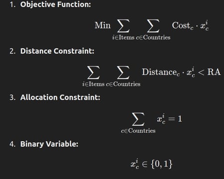
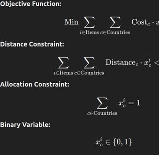
The distances between the predicted series values and the closest cluster trained in the SOM were used as risk parameters. These risk parameters were then integrated into an optimization model that employs linear programming to minimize costs while maintaining a specified risk level—categorized as high, medium, or low. This approach allows for a balanced trade-off between cost efficiency and risk management, ensuring that the optimization aligns with the desired risk tolerance levels. 

Below is the model used for this optimization:

We primarily utilized AWS Lambda for both the training and inference layers of the model, mainly due to its cost-effectiveness and "pay as you go" pricing model. AWS Lambda allowed us to efficiently manage resources without incurring unnecessary expenses.

Additionally, we used an EC2 instance solely to host the frontend, providing a stable and scalable environment for user interaction. This combination of technologies ensured a streamlined and cost-efficient solution that met the project's needs effectively.

Software Engineering

Technology Selection and Explanation

Backend Development

The diagram above illustrates both our ETL pipeline and our application architecture. The forecasting model is composed of two Lambda functions. One function performs individual forecasts, while the other, called "execute," retrieves all the necessary values from the Data Warehouse (DW) to generate the predictions. The "execute" function utilizes threading to take advantage of the parallelization capabilities of Lambda, ensuring efficient processing and faster execution times. This setup allows us to maximize performance and scalability in our backend processes.

We used Streamlit for the frontend development, primarily because it is a Python-integrated tool that provides easy access and a straightforward workflow for creating product prototypes. Streamlit allowed us to rapidly develop and deploy a user interface that interacts seamlessly with our Python-based backend. Additionally, the frontend includes a cost optimization model that considers risk constraints, offering a user-friendly way to interact with the system and make informed decisions based on the forecasts and optimizations provided by the backend.

Project
Deployment

Frontend Development

Given our decision to use AWS Lambda for deployment, we utilized Pants to build our applications and generate Docker images. These Docker images were subsequently pushed to Amazon Elastic Container Registry (ECR). This approach allowed us to efficiently manage our deployment pipeline, ensuring that our applications are containerized and ready for deployment in a scalable and manageable way using AWS services.